Snapping Points (USGS Gages) to Lines (Rivers) and Calculate Distances Along Lines

This may seem a fairly straight forward task, and it does use some relatively simple geospatial operations, but collectively I found this to be a bit trickier to do (in R). I wanted to post something here that would provide some examples of how to do this, since I need to do things like this quite often. There are probably several ways to do this, but I’ll show one option, mainly using {sf}. There are some interesting and rather annoying precision issues that crop up when doing this, so you’ll see the work around I’ve used below. A fair amount of googling and checking SO found that there are many who have run into this precision issue, so be kind to yourself!

I’m using a couple great packages here that will help use do a few things (including calculate distances along a line…see the next tutorial for more info). Namely, {nhdplusTools}, which is an immensely useful and powerful package for any person working with hydrology/river/streams (or wanting to make a map with river lines on it). In addition, we’ll need some of the other usual suspects:

library(sf) # spatial operations
library(mapview) # html mapping
library(leaflet) # html mapping
library(ggplot2) # plotting
library(dplyr) # wrangling data
library(here) # setting directories safely
library(viridis) # color scheme
library(USAboundaries) # county/state boundaries
library(nhdplusTools) # USGS/NHD rivers data

Important, before proceeding, you’ll want to make sure you’re connected to the internet. In addition, there have been some issues with downloading {nhdplusTools} data from webservers, so if it doesn’t work, try again later. Note: if you want to skip downloading data via {nhdplusTools}, all required data from this post is here if you want to download and unzip. Skip to [Snapping Points to Lines]

Get Data: Using {nhdplusTools}

First, let’s pick a single point (lat/lon), and make it spatial, and then show how we can use that point to download river lines upstream and downstream of that point, and search for USGS gages along the streamlines associated with this point. Let’s pick a point in one of the most beautiful National Parks, Yosemite! Once we have a point that is now “spatial” (see class()), we can use the {nhhplusTools} package to look up the nearest comid, which is the NHD ID for a single stream segment.

library(nhdplusTools)

# create a point in yosemite valley
yose <- st_sfc(st_point(c(-119.60020, 37.73787)), crs = 4326)

# check class is "sfc" and "sfc_POINT"
class(yose)

## [1] "sfc_POINT" "sfc"

# now figure out the nearest stream segment ID to our point
(yose_comid <- discover_nhdplus_id(yose))

## [1] 21609461

Great, so we can use the comid=21609461 to look up and download streamlines (or “flowlines”) for our area of interest, both upstream and downstream. First, let’s use a handy function in {nhhplusTools} which allows us to look up and see what data is available for our comid.

# first make a list defining the sourcetype and ID
yose_list <- list(featureSource="comid", featureID=yose_comid)

Download Flowline Data

Once we know there are data available upstream and downstream, and we have a starting comid, we can move forward and download some flowline data. Here we’ll start with all the upstream segments (everything that flows into the selected stream segment we identified). We can specify a distance we want to keep our search within (so only get flowlines that extend a set distance away from our point/segment), but don’t do that here. Importantly, we need to specify data_source = "" to force the function to search and download the data from the web. Here we download the upstream and downstream flowlines, but for downstream, we specify only the “mainstem”, which in this case is the Merced River.

• DM = “Downstream Mainstem”, UM = “Upstream Mainstem”, UT = “Upstream Tributaries”

Finally, if we want to download this data as a geopackage that we can use locally, we can use a list of all the comids and download the data using the handy subset_nhdplus function. Be aware that if you are downloading large areas of data, this can take a second, and can be large in size. However, generally it’s much smaller and faster than the entire NHDPlus dataset which is over 15 GB in size for the entire USA.

Code

# get upstream flowlines
yose_us_flowlines <- navigate_nldi(nldi_feature = yose_list,
                                   mode="UT",
                                   data_source = "")


# get downstream mainstem only (from our starting segment):
yose_ds_flowlines <- navigate_nldi(nldi_feature = yose_list, 
                             mode = "DM", 
                             #distance_km = 50,
                             data_source = "")


# make a list of all the comids we've identified:
all_comids <- c(yose_us_flowlines$nhdplus_comid, yose_ds_flowlines$nhdplus_comid)

# download all data and create a geopackage with the comid list
yose_gpkg <- subset_nhdplus(comids=all_comids,
                              simplified = TRUE,
                              overwrite = TRUE,
                              output_file = paste0(here::here(), "/data/yose_nhdplus.gpkg"),
                              nhdplus_data = "download",
                              return_data = FALSE)

# check layers in database:
st_layers(paste0(here::here(), "/data/yose_nhdplus.gpkg"))

# pull the flowlines back in
yose_streams <- read_sf(paste0(here::here(), "/data/yose_nhdplus.gpkg"), "NHDFlowline_Network")

Let’s take a look at what we’ve got so far, using some basic mapping options and the {sf} package.

Code

# make a map
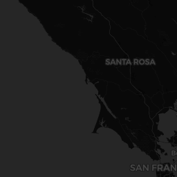
prettymapr::prettymap({
  rosm::osm.plot(project = FALSE, 
                 bbox = matrix(st_bbox(yose_streams), byrow = FALSE, ncol = 2, 
                               dimnames = list(c("x", "y"), c("min", "max"))), 
                 type = "cartolight", quiet = TRUE, progress = "none")
  plot(yose_streams$geom, col = "steelblue", lwd = (yose_streams$streamorde / 4), add=TRUE)
  plot(yose, add=TRUE, pch=21, bg="orange", cex=1.5)
  prettymapr::addnortharrow()
})

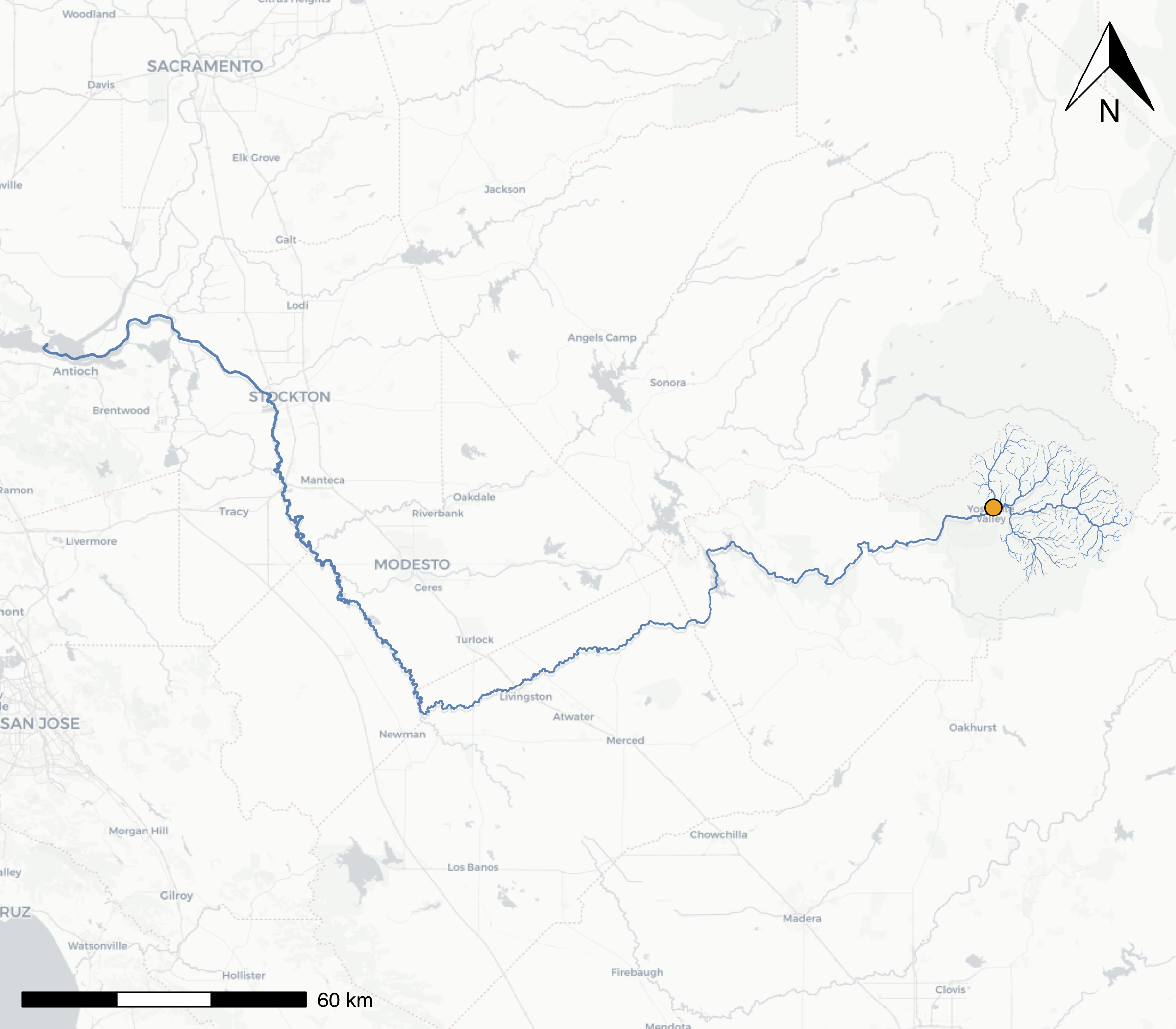
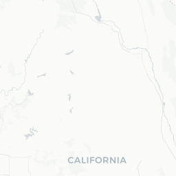
A map of the mainstem Merced River flowing into the San Joaquin, with all headwater tributaries that flow into Yosemite Valley at our selected comid river segment (orange dot). The line width of the streamlines have been scaled by the stream order

Find & Download Nearby USGS Gages

Now that we have flowlines, we can search along these flowlines for any USGS gage locations. We’ll use these to snap points to lines, and then calculate distances along these lines. First we look at upstream flowlines…and find one gage! Let’s use that gage to search downstream, just as an example of using gages or comids to search/download data.

Code

# find upstream gages
yose_us_gages <- navigate_nldi(yose_list,
              mode = "UT",
              data_source = "nwissite")

# get downstream everything from our only upstream gage (Happy Isles)
usgs_point <- list(featureSource="nwissite", featureID = "USGS-11264500")

# find all downstream gages on the mainstem river (Merced/San Joaquin)
yose_ds_gages <- navigate_nldi(yose_list,
              mode = "DM",
              #distance_km = 50,
              data_source = "nwissite",
              )

# let's add these data to our geopackage as well
# remember it's best to have everything in the same projection
st_crs(yose_streams)==st_crs(yose_us_gages)

# write to geopackage: overwite the layer if it exists
st_write(yose_us_gages, dsn=paste0(here::here(),"/data/yose_nhdplus.gpkg"), 
         layer="yose_us_gages", append = FALSE, delete_layer = TRUE)

st_write(yose_ds_gages, dsn=paste0(here::here(),"/data/yose_nhdplus.gpkg"), 
         layer="yose_ds_gages", append = FALSE, delete_layer = TRUE)

# check layers:
st_layers(paste0(here::here(), "/data/yose_nhdplus.gpkg"))

Let’s take a quick look at our data now using an interactive map with the {mapview} package. Here flowline color is scaled by the stream order (stream size).

Code

m1 <- mapview(yose, col.regions="black", cex=6, layer.name="Start Point") + 
  mapview(yose_streams, zcol="streamorde", legend=TRUE, layer.name="Stream <br> Order") + 
  mapview(yose_us_gages, col.regions="orange", layer.name="U/S Gage") +
    mapview(yose_ds_gages, col.regions="maroon", layer.name="D/S Gages")

# add a measurement tool
m1@map %>% leaflet::addMeasure(primaryLengthUnit = "kilometers") %>%
  leaflet.extras::addFullscreenControl(position = "topleft")

+−

CartoDB.Positron

CartoDB.DarkMatter

OpenStreetMap

Esri.WorldImagery

OpenTopoMap

Start Point

Stream
Order

U/S Gage

D/S Gages

Stream
Order

1
2
3
4
5
6
7

U/S Gage

D/S Gages

Measure

Measure distances and areas

Create a new measurement

Measure distances and areas

Start creating a measurement by adding points to the map

• Cancel
• Finish measurement

Zoom full

30 km

30 mi

D/S Gages

U/S Gage

Stream
Order

Start Point

Leaflet | © OpenStreetMap contributors © CARTO

Mapview1

Get Euclidean Distances between Gages

If we want to do a quick approximation of distances between points, there are some quick tools we can use. This is mainly to demonstrate these tools functionality, as you can see the actual river distance is likely much larger than what is calculated here. We’ll use this to compare with the next section.

Here we can use nearest neighbor distances to calculate euclidean distances between points (or USGS gages in our example). The {nngeo} package and the nn2 function are one good way to do this. First we need to project our data, since the nn2 requires projected data. Then we can use our interactive map above and click on the most downstream point to find out what the gage ID is (USGS-11337190). We’ll use this to assess how far the most downstream gage is from the most upstream gage in our dataset.

# need these
library(nngeo)

# Project first (to ensure using nngeo::nn2, otherwise lat/lon is similar to st_distance)
merced_us_gage <- st_transform(yose_us_gages, 26910)

# get the most downstream gage (find ID using mapview map)
merced_ds_gage <- yose_ds_gages %>% filter(identifier=="USGS-11337190") %>% st_transform(26910)

# calculate the max euclidean (straight line) distance in meters
max_gage_dist <- st_nn(merced_ds_gage, merced_us_gage, returnDist = TRUE, progress = FALSE) 

# now convert this measurement to km
measurements::conv_unit(max_gage_dist$dist[[1]], "m", "km")

## [1] 190.7227

Measuring the same distance between our most upstream USGS gage (Happy Isles) and the most downstream gage (San Joaquin at Jersey Point), I got a distance of 190.7 km. So all in all, I’d say we are doing well. The difference is likely due to slight differences in the projection of the mapview map as well as any innaccuracies associated with where we clicked on the points on the map. Let’s move on and try to do this using the actual river distance (along the flowlines).

Snap Points to Lines

Great, now let’s snap our points to lines, and then calculate the river distance between the most upstream and most downstream USGS gage. First, because of some interesting issues relating to precision and rounding, even though we think our points may be on a line, in actuality, they may not be. Check out this Stack Overflow thread. The basic premise is that even if a point is infinitesimally close to a line, it may look like it intersects with the line, but in fact there is some tolerance or precision level that negates this. The easiest work-around is to buffer or adjust the tolerance of the intersection, so that the point will indeed intersect with the line.

Let’s take a look at our USGS gage points we grabbed in the code above so we can demonstrate this issue, and one possible solution.

st_snap_points <- function(x, y, namevar, max_dist = 1000) {
  
  # this evaluates the length of the data
  if (inherits(x, "sf")) n = nrow(x)
  if (inherits(x, "sfc")) n = length(x)
  
  # this part: 
  # 1. loops through every piece of data (every point)
  # 2. snaps a point to the nearest line geometries
  # 3. calculates the distance from point to line geometries
  # 4. retains only the shortest distances and generates a point at that intersection
  out = do.call(c,
                lapply(seq(n), function(i) {
                  nrst = st_nearest_points(st_geometry(x)[i], y)
                  nrst_len = st_length(nrst)
                  nrst_mn = which.min(nrst_len)
                  if (as.vector(nrst_len[nrst_mn]) > max_dist) return(st_geometry(x)[i])
                  return(st_cast(nrst[nrst_mn], "POINT")[2])
                })
  )
  # this part converts the data to a dataframe and adds a named column of your choice
  out_xy <- st_coordinates(out) %>% as.data.frame()
  out_xy <- out_xy %>% 
    mutate({{namevar}} := x[[namevar]]) %>% 
    st_as_sf(coords=c("X","Y"), crs=st_crs(x), remove=FALSE)
  
  return(out_xy)
}

Snap USGS Gages to Flowlines

Let’s see how we can implement this with our gages. Make sure load the function by running the chunk, and then proceed below. First we need to bind our gage data into one dataframe, it will make things easier when we move forward.

Code

# first lets merge all our gages into one dataframe. Make sure in same crs
st_crs(yose_us_gages)==st_crs(yose_ds_gages)

## [1] TRUE

Code

# now bind together
all_gages <- rbind(yose_us_gages, yose_ds_gages) 

# check for duplicates (should be n=14)
all_gages %>% distinct(identifier) %>% nrow()

## [1] 14

Sidenote: Sometimes you may get an error here (when binding two sf dataframes). It happens to me frequently. When merging or binding to datasets together, both of which are spatial (sf), if the column names don’t match exactly, or the CRS is different, you may run into this. It’s straightforward to fix! Make sure columns are identical before using rbind. If you have different numbers of columns (but the geometry column and crs is identical in each dataframe), it’s possible to use this nifty {data.table} trick as well. It will fill any columns that don’t match with NAs.

Code

# try using different numbers of cols in each dataframe (but keep geom in both)
all_gages <- st_as_sf(data.table::rbindlist(
   list(yose_us_gages[,c(2,6,8)], yose_ds_gages), fill = TRUE))

# note there are NAs in the columns that were missing from the yose_us_gage dataframe.

Ok, now we can use our custom function to snap our USGS gages to our flowline, using a buffer of 100 meters. We need to project our data here for this to work correctly.

Code

# first project
all_gages_proj <- st_transform(all_gages, crs = 26910)
yose_streams_proj <- st_transform(yose_streams, crs=26910)

# now snap points to the lines using a 500 meter buffer, select which ID column you want keep for rejoining
gages_snapped <- st_snap_points(all_gages_proj, yose_streams_proj, namevar = "identifier", max_dist = 500)

Great, that seemed to work but let’s take a look at our gages and see if they are indeed “snapped” to the flowline. Zoom in close enough and you should see that our points have indeed been shifted to exactly intersect with the nearest point on the flowline.

Code

mapview(gages_snapped, col.regions="cyan", layer.name="Snapped Gages") +
  mapview(yose_streams_proj, color="steelblue", layer.name="Flowlines") + 
  mapview(all_gages, col.regions="orange", layer.name="All Gages")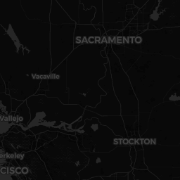

+−

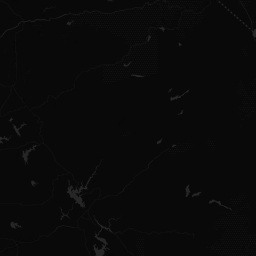
CartoDB.DarkMatter

CartoDB.Positron

OpenStreetMap

Esri.WorldImagery

OpenTopoMap

Snapped Gages

Flowlines

All Gages

Snapped Gages

Flowlines

All Gages

Zoom full

30 km

30 mi

All Gages

Flowlines

Snapped Gages

Leaflet | © OpenStreetMap contributors © CARTO

Let’s zoom in on our Happy Isles gage to get a better sense of what we’ve done. Here we should see the gage has been snapped to the line.

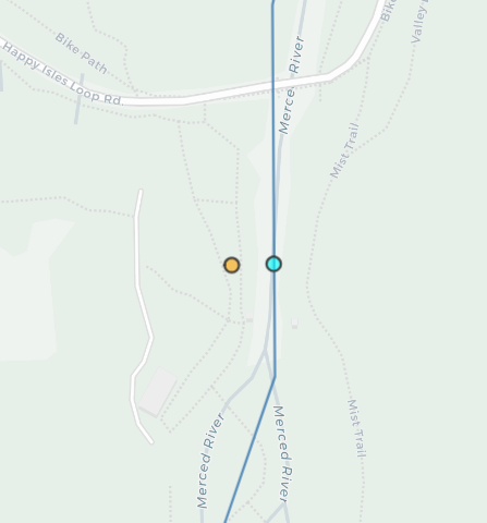
Snapped points in bright cyan are now aligned to the flowline, while the original gage location is slightly off of the channel.

Split Segments by Points

If you’ve made it this far congrats! you are in the home stretch. The next task which is sometimes required, is to split our line or lines at the point locations. In this case, if we want to calculate exactly how far the river distance is from our most upstream gage (Happy Isles) to our most downstream gage (San Joaqin-Jersey Point), we need to split our flowlines at each gage intersection point.

Again, this means we need to make sure our point actually intersect the lines. One quick work around here is to use a buffer to intersect points with lines, and then use that intersection to split the lines. We need the {lwgeom} package here, which took a bit of sleuthing to make sure it was installed properly. Check the {sf} website and the {lwgeom} website.

library(lwgeom)

# create a 1 meter buffer around snapped point
gages_snapped_buff <- st_buffer(gages_snapped, 1)

# now use lwgeom::st_split to split stream segments
segs <- st_collection_extract(lwgeom::st_split(yose_streams_proj, gages_snapped_buff), "LINESTRING") %>% 
  tibble::rownames_to_column(var = "rowid") %>% 
  mutate(rowid=as.integer(rowid))

And as always, let’s visualize what we did. First let’s filter to just the mainstem Merced and San Joaquin…this took a little playing around to get the right filter set up.

# filter to only the mainstem Merced or San Joaquin 
segs_filt <- segs %>% filter(gnis_name %in% c("Merced River", "San Joaquin River") |
                               comid %in% c(21609445, 21609461)) %>% 
                               filter(ogc_fid <= 2621772 | streamorde > 4)

Then we can map!

mapview(segs_filt, zcol="gnis_name")  + mapview(segs, color="blue", lwd=0.3) +
  mapview(gages_snapped, col.regions="cyan", layer.name="Snapped Gages")

+−

CartoDB.Positron

CartoDB.DarkMatter

OpenStreetMap

Esri.WorldImagery

OpenTopoMap

segs_filt - gnis_name

segs

Snapped Gages

segs_filt - gnis_name

Merced River
San Joaquin River

segs

Snapped Gages

Zoom full

30 km

30 mi

Snapped Gages

segs

segs_filt - gnis_name

Leaflet | © OpenStreetMap contributors © CARTO

Calculate River Distances

Now we can calculate the distances between each gage. Here we drop a few loose ends (segments on either end of the most upstream/downstream gages), then we calculate the length of each line segment, then arrange by the hydroseq (a sequential ID for stream flow), and use that to calculate a cumulative distance from the upstream point to the downstream point!

segs_filt_dist <- segs_filt %>% 
  # drop the "loose ends" on either extent (upstream or downstream) of first/last gage
  filter(!rowid %in% c(232, 100, 66, 62, 63)) %>% 
    mutate(seg_len_m = units::drop_units(units::set_units(st_length(.), "m")),
         seg_len_km = seg_len_m/1000) %>% 
  arrange(desc(hydroseq)) %>% 
  mutate(total_len_km = cumsum(seg_len_km)) %>% 
  # filter to just cols of interest
  select(rowid, ogc_fid:comid, gnis_id:reachcode, streamorde, hydroseq, seg_len_km, total_len_km, geom)

# filter to just upstream and just downstream gages:
gages_snapped_usds <- filter(gages_snapped, identifier %in% c("USGS-11337190", "USGS-11264500"))

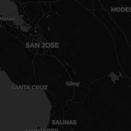
mapview(segs_filt_dist, zcol="total_len_km", layer.name="Cumulative Flowline<br> Distance (km)")  +
  mapview(gages_snapped_usds, zcol="identifier", layer.name="USGS Gages")

+−

CartoDB.Positron

CartoDB.DarkMatter

OpenStreetMap

Esri.WorldImagery

OpenTopoMap

Cumulative Flowline
Distance (km)

USGS Gages

Cumulative Flowline
Distance (km)

USGS Gages

USGS-11264500
USGS-11337190

Zoom full

30 km

30 mi

USGS Gages

Cumulative Flowline
Distance (km)

Leaflet | © OpenStreetMap contributors © CARTO

So the final answer is a total distance of 375.97 km between our most upstream gage in the Merced, and the most downstream gage (in the San Joaquin). That’s a long ways! And that is also nearly twice what we estimated using our euclidean straight line method earlier.

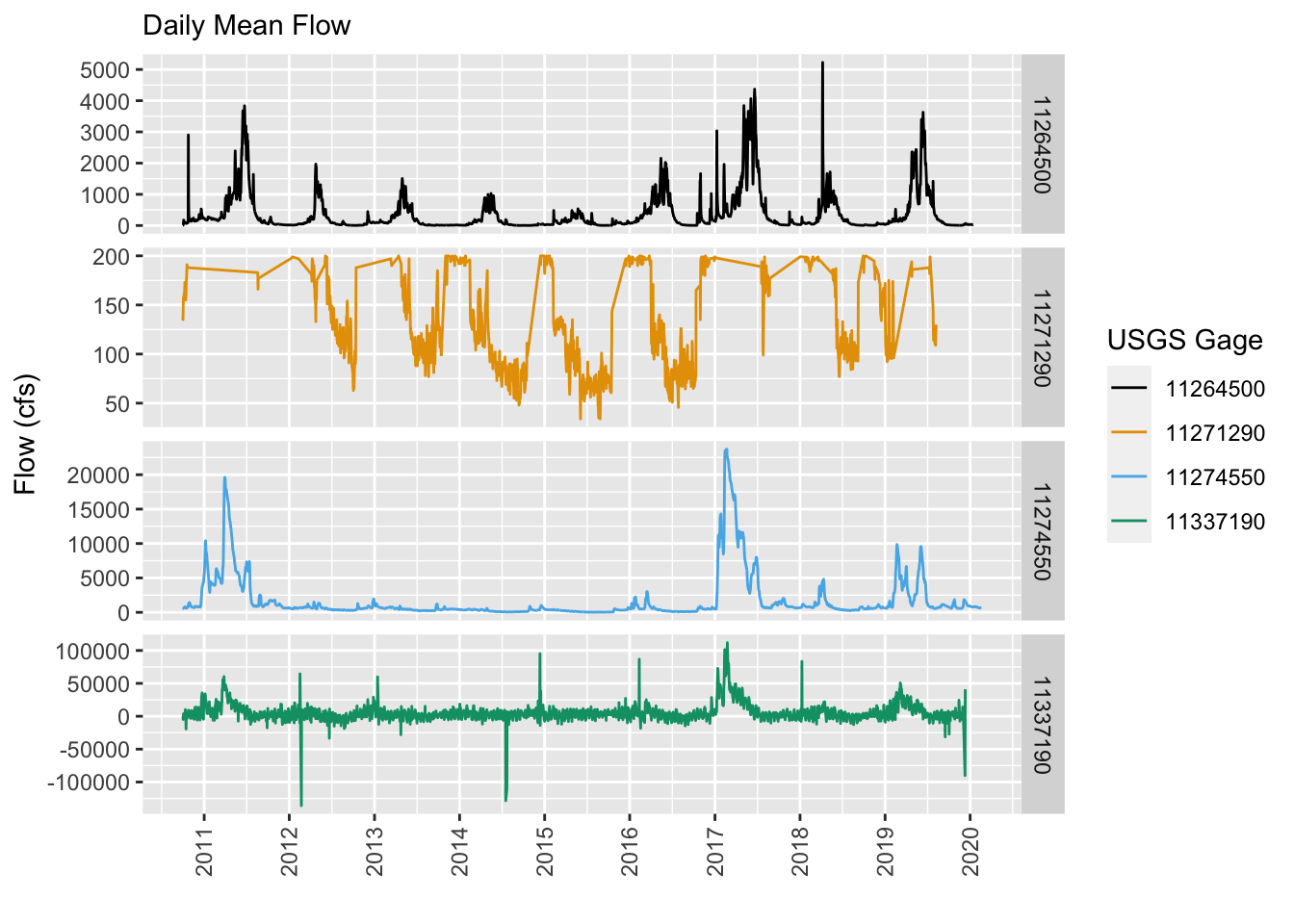
BONUS: Compare Gage Flow in Each Gage

Just out of curiosity, let’s see what flows look like at a few of these gages. Let’s take 2 from the San Joaquin and 2 from the Merced. Let’s use the great USGS dataRetrieval package to grab the most recent flow data and compare. Can you guess by looking at these plots which is the most downstream and which is the most upstream gage? Negative flow values! What could that mean!? :)