Using Shapefiles with sf

There are loads of spatial mapping/plotting packages in R. The primary way to read in spatial data is with the sf package. Let’s look at how to load/plot line and polygon data.

Let’s load packages first:

library(tmap)
library(tmaptools)
library(purrr)
library(dplyr); # wrangling data/plotting
library(readr);
library(viridis); # nice color palette
library(sf); # newer "simple features" spatial package
library(USAboundaries); # state/county data
#library(Imap); # nice mapping/color functions col.map
library(ggrepel) # for labeling

Polyline/Polygons Shapefile Data

I’ve downloaded some HUC watershed boundaries from the Lake Tahoe area in California, they are here on github. Download the zipped file and unzip it in a data folder. We’re going to use shapefiles for the remainder of this example. ### Load shapefiles with sf

Here’s how to do the same thing using the sf package. Notice one important points about sf…sticky geometry!

• the sf package reads things in as a regular dataframe, with the spatial component of the data contained inside a geometry list-column within the dataframe. That means you can operate on this data as you would any data frame, because the geometry column will always stick with the data.

# notice the simple structure, but results in dataframe
hucs_sf <- st_read("data/h8_tahoe.shp") # fast!

## Reading layer `h8_tahoe' from data source `/Users/rapeek/Documents/github/mapping-in-R-workshop/data/h8_tahoe.shp' using driver `ESRI Shapefile'
## Simple feature collection with 1 feature and 5 fields
## Geometry type: POLYGON
## Dimension:     XY
## Bounding box:  xmin: -120.2525 ymin: 38.7041 xmax: -119.877 ymax: 39.32512
## Geodetic CRS:  WGS 84

# check crs
st_crs(hucs_sf)

## Coordinate Reference System:
##   User input: WGS 84 
##   wkt:
## GEOGCRS["WGS 84",
##     DATUM["World Geodetic System 1984",
##         ELLIPSOID["WGS 84",6378137,298.257223563,
##             LENGTHUNIT["metre",1]]],
##     PRIMEM["Greenwich",0,
##         ANGLEUNIT["degree",0.0174532925199433]],
##     CS[ellipsoidal,2],
##         AXIS["latitude",north,
##             ORDER[1],
##             ANGLEUNIT["degree",0.0174532925199433]],
##         AXIS["longitude",east,
##             ORDER[2],
##             ANGLEUNIT["degree",0.0174532925199433]],
##     ID["EPSG",4326]]

Polygon Shapefile Data

No different here, process is the same. But let’s take a look at a package that might be helpful for folks working with state/county boundaries.

Download State/County Data

A nice package for pulling county/state data is the urbnmapr package. Importantly, this package pulls these data in as sf features (dataframes), not as rgdal or SpatialPolygonDataFrames data.

Let’s show this in two steps, the first is how to grab a sf feature for a given state or states.

library(urbnmapr)

# Pick a State
state_names <- c("CA")

# warning is ok
CA <- get_urbn_map(map = "states", sf = TRUE) %>% filter(state_abbv==state_names)

## old-style crs object detected; please recreate object with a recent sf::st_crs()

st_crs(CA)

## Coordinate Reference System:
##   User input: EPSG:2163 
##   wkt:
## PROJCRS["NAD27 / US National Atlas Equal Area",
##     BASEGEOGCRS["NAD27",
##         DATUM["North American Datum 1927",
##             ELLIPSOID["Clarke 1866",6378206.4,294.978698213898,
##                 LENGTHUNIT["metre",1]]],
##         PRIMEM["Greenwich",0,
##             ANGLEUNIT["degree",0.0174532925199433]],
##         ID["EPSG",4267]],
##     CONVERSION["US National Atlas Equal Area",
##         METHOD["Lambert Azimuthal Equal Area (Spherical)",
##             ID["EPSG",1027]],
##         PARAMETER["Latitude of natural origin",45,
##             ANGLEUNIT["degree",0.0174532925199433],
##             ID["EPSG",8801]],
##         PARAMETER["Longitude of natural origin",-100,
##             ANGLEUNIT["degree",0.0174532925199433],
##             ID["EPSG",8802]],
##         PARAMETER["False easting",0,
##             LENGTHUNIT["metre",1],
##             ID["EPSG",8806]],
##         PARAMETER["False northing",0,
##             LENGTHUNIT["metre",1],
##             ID["EPSG",8807]]],
##     CS[Cartesian,2],
##         AXIS["easting (X)",east,
##             ORDER[1],
##             LENGTHUNIT["metre",1]],
##         AXIS["northing (Y)",north,
##             ORDER[2],
##             LENGTHUNIT["metre",1]],
##     USAGE[
##         SCOPE["Statistical analysis."],
##         AREA["United States (USA) - onshore and offshore."],
##         BBOX[15.56,167.65,74.71,-65.69]],
##     ID["EPSG",9311]]

That was easy…what about counties? We can use the same type of call, but let’s add some dplyr and purrr functionality here to add the X and Y values for the centroid of each polygon (county) we download. In this case we use map_dbl because it will take a vector or values (the geometry col here), map a function over each row in that vector, and return a vector of values (the centroid points).

library(purrr)

# Pick some CA counties
co_names <- c("Butte County", "Placer County", 
              "El Dorado County", "Nevada County", 
              "Yuba County", "Sierra County",
              "Plumas County")

# get counties
counties_spec <- get_urbn_map(map = "counties", sf=TRUE) %>% 
  filter(state_abbv==state_names, county_name %in% co_names)

## old-style crs object detected; please recreate object with a recent sf::st_crs()

# add centroid for each county using purrr::map_dbl
counties_spec <- counties_spec %>% 
  mutate(lon = map_dbl(geometry, ~st_centroid(.x)[[1]]),
         lat = map_dbl(geometry, ~st_centroid(.x)[[2]]))

Make a Basic Map

First let’s show a few examples comparing how to plot the dataset using sf.

plot(st_geometry(hucs_sf), col="darkblue", 
     main="Tahoe HUC8", axes=TRUE)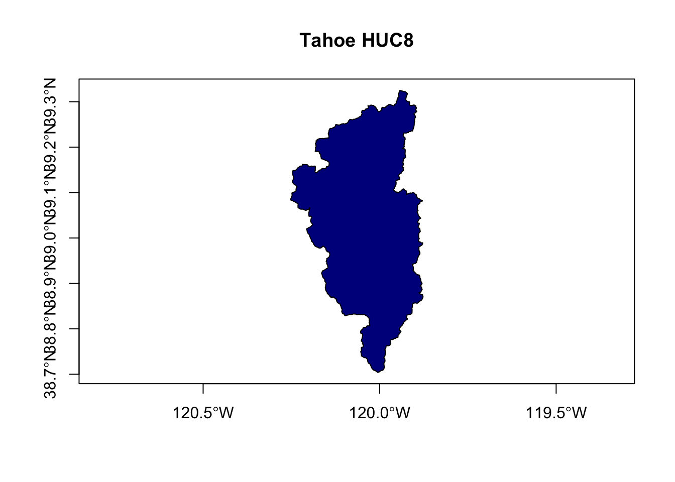

# this is same
# plot(hucs_sf$geometry), col="darkblue", main="Tahoe HUC8")

Advanced Mapping

Okay, let’s add in the county/state data, and figure out a few tricks to making our map a bit cleaner.

Layering Maps: plot and sf

# note adding some alpha adjustment here and using "cex" to make larger
plot(counties_spec$geometry, col=adjustcolor("maroon", alpha=0.5), cex=1.5, axes=TRUE, main="Selected CA Counties")

# now add tahoe HUC8 to existing plot, with add=TRUE
plot(hucs_sf$geometry, col=adjustcolor("blue", alpha=0.7), add=TRUE)

# now add some labels using the centroid lat/long we added earlier
text(counties_spec$lon, counties_spec$lat, labels = counties_spec$name)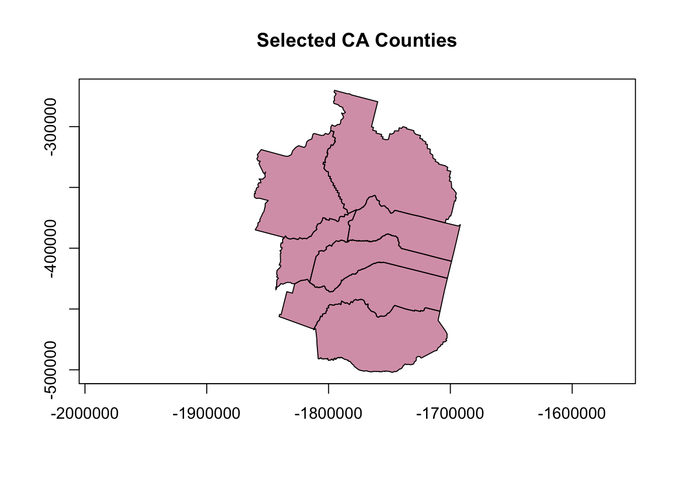

Unforunately this map isn’t very good. How can we improve it? Seems it would be nicer to crop the river layer to the counties of interest, or at least center things on that area. Also might be nice to have the labels on top and not obscured by the rivers.

# get range of lat/longs from counties for mapping
mapRange1 <- st_bbox(counties_spec) # view bounding box

# add counties
plot(counties_spec$geometry, col=adjustcolor("maroon", alpha=0.5), cex=1.5,
     xlim=mapRange1[c(1,3)], ylim = mapRange1[c(2,4)], axes=TRUE, 
     main="Selected CA Counties and Tahoe HUC8")

# add HUC
plot(hucs_sf$geometry, col=adjustcolor("blue", alpha=0.7), add=TRUE)
     
# add labels for counties
text(counties_spec$lon, counties_spec$lat, labels = counties_spec$name,
     col=adjustcolor("white", alpha=0.8), font = 2)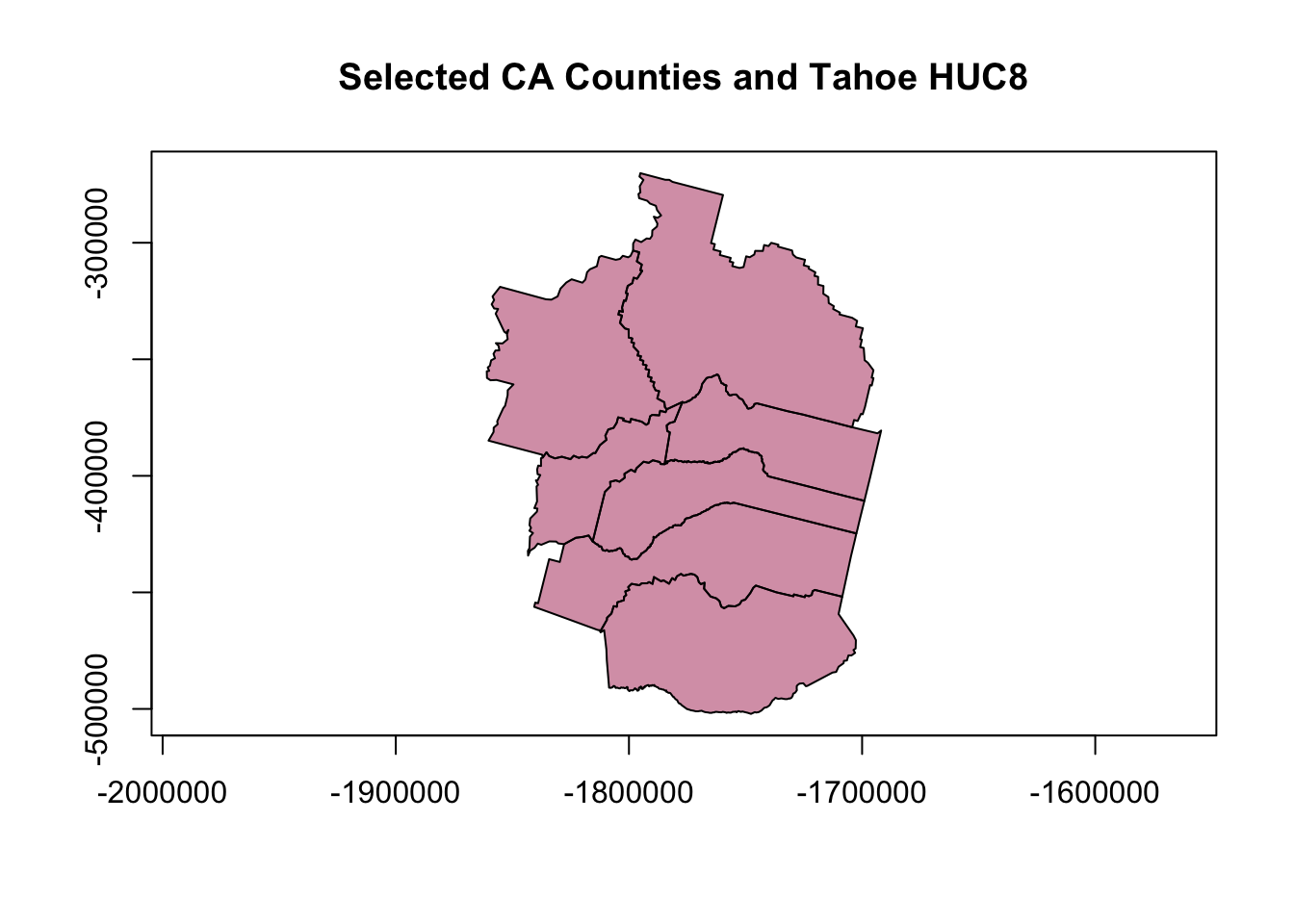

That’s a little better…but still not quite what we want. Lots of extra ink going toward stuff that we don’t need (i.e., watershed boundary outside of counties). What about cropping the watershed layer to our county layer (just for fun)?

Cropping & Buffering with sf

Great thing is that sf has some really nice tools for this, just as any GIS program would. Here let’s use st_intersection to crop our watershed layer to only include the part inside the counties of interest.

# need to make sure CRS is the same!
st_crs(hucs_sf)==st_crs(counties_spec)

## [1] FALSE

counties_spec <- st_transform(counties_spec, st_crs(hucs_sf))

# crop watershed by counties
hucs_sf_crop <- st_intersection(hucs_sf, counties_spec) # warning is ok

## Warning: attribute variables are assumed to be spatially constant throughout all geometries

# plot
plot(hucs_sf_crop$geometry, col="blue") # a quick plot check to make sure it worked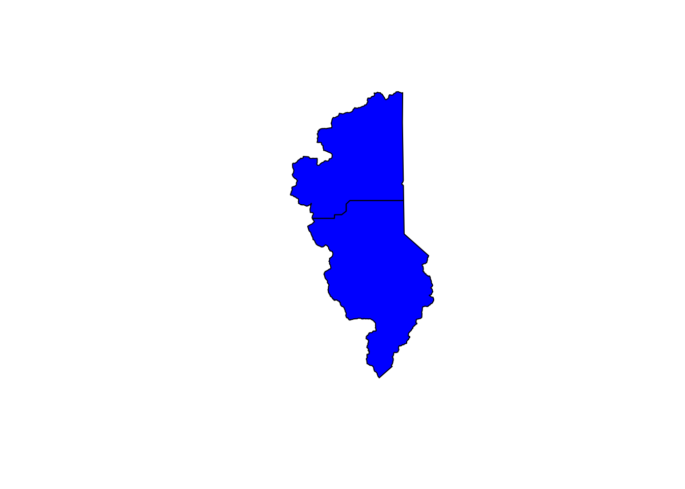

# buffer a single county? Warning is ok as well...has to do with lat/lon
county_buff <- st_buffer(counties_spec[counties_spec$name=="El Dorado",], dist = .05) # note this is a buffer of decimal degrees

# now plot
plot(counties_spec$geometry, axes=TRUE)
plot(county_buff$geometry, border="maroon", col=adjustcolor("maroon", alpha=0.5), add=TRUE)
plot(hucs_sf_crop$geometry, col="blue", add=TRUE)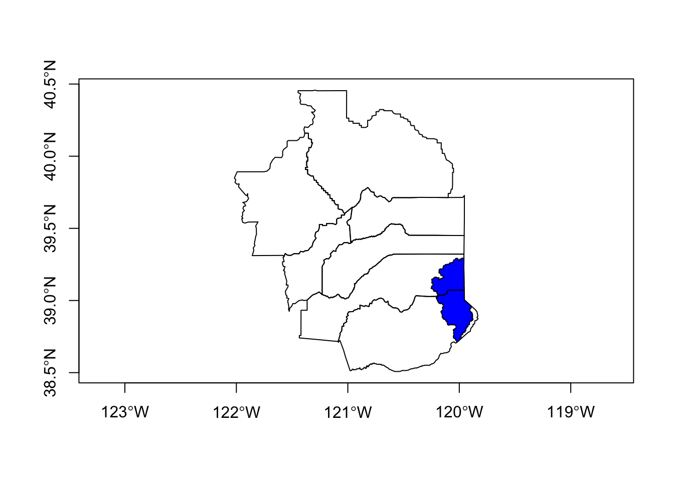

Great, let’s try our plot again.

# try again, let's switch layer ordering
plot(counties_spec$geometry, col=adjustcolor("maroon", alpha=0.2), cex=1.5, axes=TRUE, main="Selected CA Counties")
plot(hucs_sf_crop$geometry, col=adjustcolor("blue", alpha=0.7),add=TRUE)
plot(CA$geometry, add=TRUE, lwd=2)
text(counties_spec$lon, counties_spec$lat, labels = counties_spec$name,
     col="maroon", font = 2)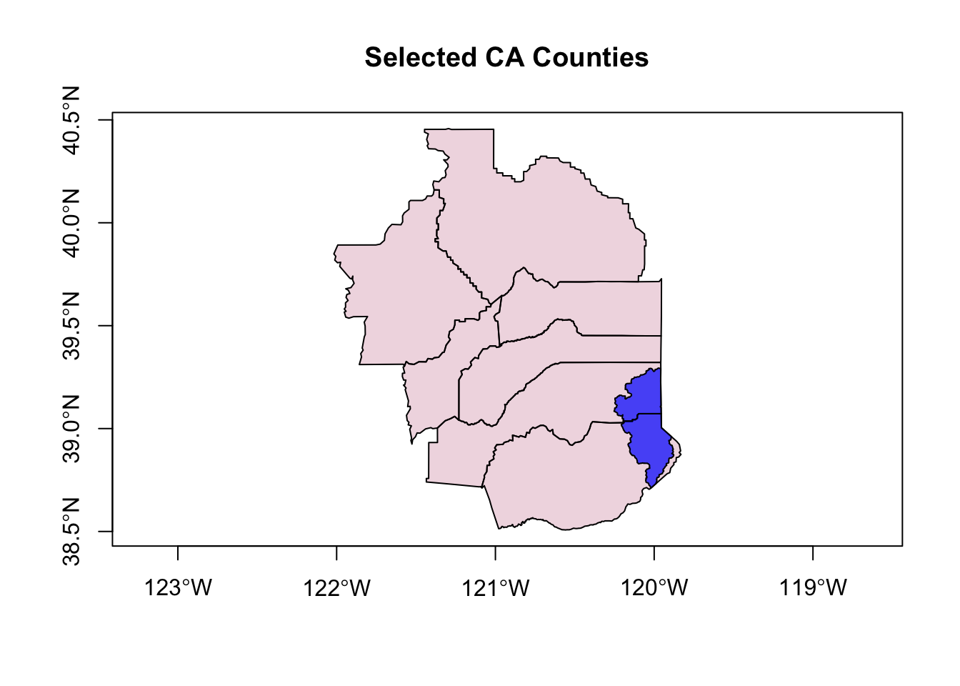

Ok! Not bad. What could we improve?

Using ggplot2 and sf

We can use ggplot2 to plot our sf data! Many more options using this platform for sf. Mapping with ggplot2 brings some extra things we can fiddle with. Since these data are all data.frames (sf features), we can use the geom_sf function.

One important note…there’s a common error that you may get semi-regularly, which will look something like this:

Error in grid.Call(C_textBounds, as.graphicsAnnot(x$label), x$x, x$y,  : 
  polygon edge not found

Don’t worry about this, it has to do with the grid package…it’s annoying but all you need to do is replot your map/figure (sometimes several times) and eventually the plot will work/show up.

library(ggplot2)
library(ggrepel)

# quick test of just CA
ggplot() + geom_sf(data = CA)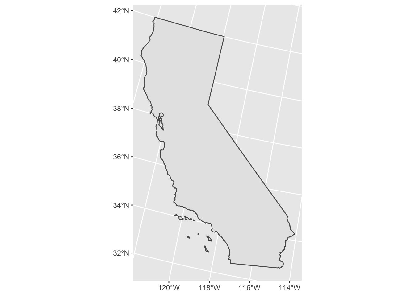

# not cropped
ggplot() + 
  geom_sf(data=CA, color = "gray30", lwd=2, fill=NA) + # California border
  geom_sf(data=counties_spec, fill = NA, show.legend = FALSE, color="gray50", lwd=0.4) + # counties
  geom_label_repel(data=counties_spec, aes(x=lon, y=lat, label=county_name)) +
  theme_bw()

## Warning: ggrepel: 1 unlabeled data points (too many overlaps). Consider increasing max.overlaps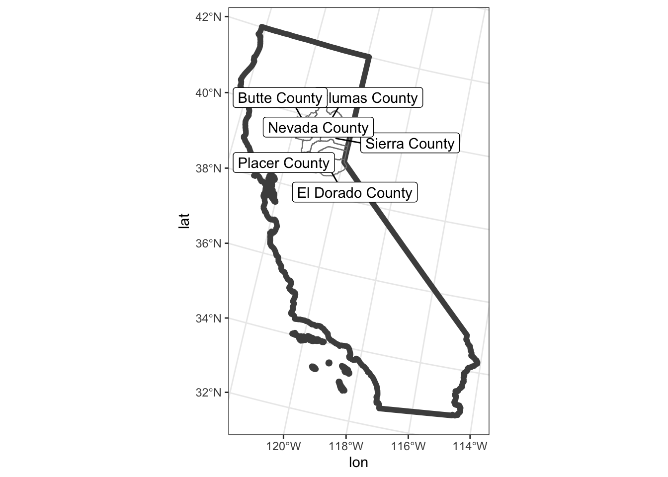

Great, this is a nice example…but what if we want to crop to the area of interest like we did previously with the st_bbox? Well, we can add a call to the coord_sf() to limit the range we’re interested in. Let’s also add an “annotation” to our map to delineate the CA state line.

# with cropped range (to only our selected counties)
ggplot() + 
  geom_sf(data=CA, color = "gray30", lwd=2, fill=NA) +
  geom_sf(data=counties_spec, fill = NA, show.legend = F, color="gray50", lwd=0.4) +
  geom_sf(data=hucs_sf_crop, fill="blue", alpha=0.5, size=0.5)+
  geom_label_repel(data=counties_spec, aes(x=lon, y=lat, label=county_name)) +
  coord_sf(xlim = mapRange1[c(1,3)], ylim = mapRange1[c(2,4)]) +
  theme_bw(base_family = "Helvetica") + # change to "sans" if this font not available
  labs(title="Selected CA Counties and Tahoe HUC8")+
  theme(panel.grid.major = element_line(color = "gray80", linetype = 1)) + # change grid
  annotate("text", x=c(-120.1,-119.9), y=40.3, label=c("CA","NV"), color="gray40", size=3, fontface=2, angle = 90)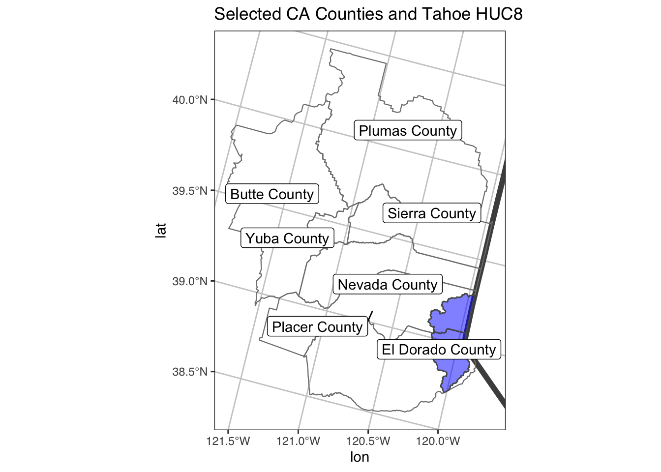

Adding a Background with tmap and tmaptools

We can use the open source tmaptools::read_osm() function to add a background map.

library(tmaptools)
library(stars)

# get extent
bbox <- st_as_sfc(st_bbox(counties_spec))

# use tmaptools to pull base layers (see ?OpenStreetMap::openmap for more options)
gm_esri <- read_osm(bbox, type = "esri-topo", raster=TRUE) # specify zoom
gm_osm <- read_osm(bbox, type = "osm", raster=TRUE) # defaults are good too
gm_hill <- read_osm(bbox, type = "stamen-toner", raster=TRUE)

# reproject
CA <- st_transform(CA, st_crs(gm_esri))

# tmap
tm1 <- tm_shape(gm_esri) + tm_rgb() +
  tm_shape(CA) + tm_polygons(border.col = "gray30", lwd=2, alpha=0) +
  tm_shape(counties_spec) + 
  tm_polygons(alpha = 0, border.col="black", lwd=1) +
  tm_text(text="county_name", shadow = TRUE, print.tiny = TRUE) +
  tm_shape(hucs_sf_crop) + tm_polygons(col="blue", alpha=0.6, size=0.5) +
  tm_layout(main.title = "Selected CA Counties and Tahoe HUC8", main.title.size = 1.2)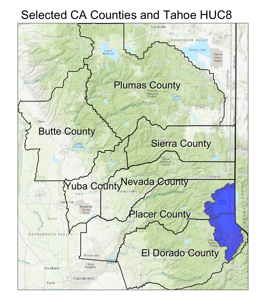

Interactive maps

We can add our sf data directly into a leaflet map using the mapview package.

library(mapview)
mapviewOptions(fgb = FALSE)

m1 <- mapview(counties_spec, fill=NA)
m2 <- mapview(hucs_sf)

# combine using the ggplot style "+"
m1 + m2

Put it All Together

• Can you crop to a single county and plot the rivers and county?
• How might you make an inset in your map? (hint…see here)
• What about buffering outside of the selected counties by 30 km?
• Can you add some points? Try adding a point at 39.4 N and 121.0 W.