Working with kml Files

The sf package can read many different file types in, and kml is no exception. The difference is kml files are the unzipped versions of kmz files. You’ll want to unzip with any sort of zip package you have on your computer (Keka, 7zip, etc.). Data used in this example live in the github repo here. Importantly, kml can contain multiple layers because they use a sort of nested format, so it’s good to check first to see which layer you may want. This example only has a single layer so we don’t need to specify a layer in our st_read function.

suppressPackageStartupMessages({
  library(ggplot2)
  library(dplyr)
  library(sf);
  library(stringi)
  })

# https://waterwatch.usgs.gov/?m=stategage

# check layers first:
st_layers("data/streamgages_06.kml")

## Driver: KML 
## Available layers:
##          layer_name geometry_type features fields
## 1 USGS streamgages       3D Point     2239      2

# read in
gages <- st_read("data/streamgages_06.kml") # reads kml but not kmz

## Reading layer `USGS streamgages ' from data source `/Users/rapeek/Documents/github/mapping-in-R-workshop/data/streamgages_06.kml' using driver `KML'
## Simple feature collection with 2239 features and 2 fields
## Geometry type: POINT
## Dimension:     XYZ
## Bounding box:  xmin: -124.2942 ymin: 32.55172 xmax: -114.1402 ymax: 42.00429
## z_range:       zmin: 0 zmax: 0
## Geodetic CRS:  WGS 84

Cleaning/Removing html tags

Once we have the data in, we still need to clean up some of the html bits that we don’t want. We can use some text/string functions to deal with this in R. gsub and substr are great functions for fixing/replacing text.

# pull out relevant info (remove html tags)
gages$name <- gsub(pattern="<.*?>", "", gages$Name)
gages$details <- gsub(pattern="<.*?>", "", gages$Description)
gages$site_no <- substr(gages$name, start = 1, stop = 8)
gages$site <- substr(gages$name, start = 10, stop = nchar(gages$name))
gages$date_s <- substr(gages$details, start=13, stop=22)
gages$date_e <- substr(gages$details, start=32, stop=nchar(gages$details)-1)
gages <- gages %>% dplyr::select(site_no:date_e)
gages$gageID <- paste0("T", gages$site_no)

# grep all sites with "AMERICAN", "DEER" or "BEAR" in site name
gages_FILTER <- filter(gages, grepl(pattern = "AMERICAN|DEER|BEAR",site))

A Basic ggplot

Here we can make a basic ggplot with no specific background to our spatial data. We can still sort of make out an outline of California, but it would be nice to add some more details.

# simple map
ggplot() +
  labs(x="Longitude (WGS84)", y="Latitude",
       title="USGS Gages in CA") + 
  geom_sf(data=gages, col="blue", lwd=0.4, pch=21) +
  theme_bw()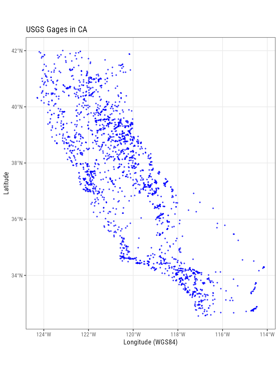

Use ggspatial for Map Background/Details

Now we can add a few additional details here. Let’s use the USAboundaries package go get a county layer, and the ggspatial package to add a scale bar, north arrow, and open source map background. Note, we could also just throw this sf layer into mapview (see the mapview page) and have an interactive map.

First let’s get the county layer:

# now with background
library(ggspatial)
library(USAboundaries)
library(purrr)

counties <- us_counties(resolution = "high", states="CA")

Next we use the ggspatial package to add background (change the zoom= to a different value to change level of detail, but beware higher values take longer to download) using the annotation_map_tile function. Then add annotation_scale and annotation_north_arrow options to make the map look complete!

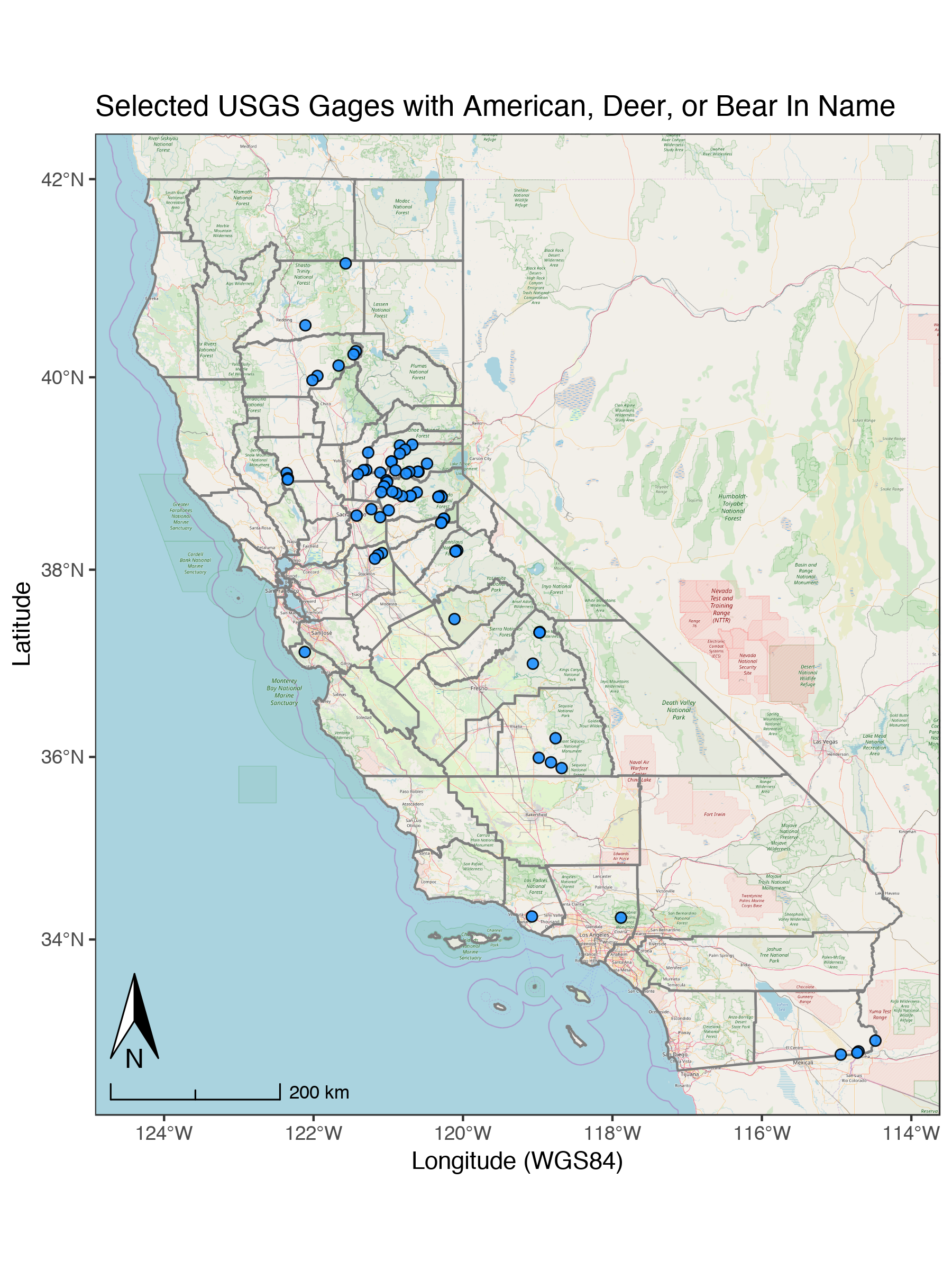
# water color version 
ggplot() +
  annotation_map_tile(zoom = 8) + # this can take a few seconds
  geom_sf(data=counties, fill=NA, col="gray50", alpha=0.7) +
  scale_color_viridis_d() +
  labs(x="Longitude (WGS84)", y="Latitude",
       title="Selected USGS Gages with American, Deer, or Bear In Name") + 
  geom_sf(data=gages_FILTER, fill="dodgerblue", alpha=0.9, pch=21, size=2) +
  # spatial-aware automagic scale bar
  annotation_scale(location = "bl",style = "ticks") +
  theme_bw() +
  # spatial-aware automagic north arrow
  annotation_north_arrow(width = unit(.3,"in"), 
                         pad_y = unit(.3, "in"),location = "bl", 
                         which_north = "true")